Julia instead of NetLogo

Simple agent-based models: NetLogo or Julia

I’m idly thinking of putting on a new computational social science module, which lead me to look at Paul Smaldino’s book, Modeling Social Behavior. This looks like a very accessible text on its title-topic. Smaldino uses NetLogo throughout, however, which I’d prefer not to do. My potential students will have been exposed to Julia, so it would be desirable to continue with that. To get an impression of the pedagogical costs of using a general rather than a domain-specific language, I decided to implement Smaldino’s first example, “particles”, from Chapter 2.

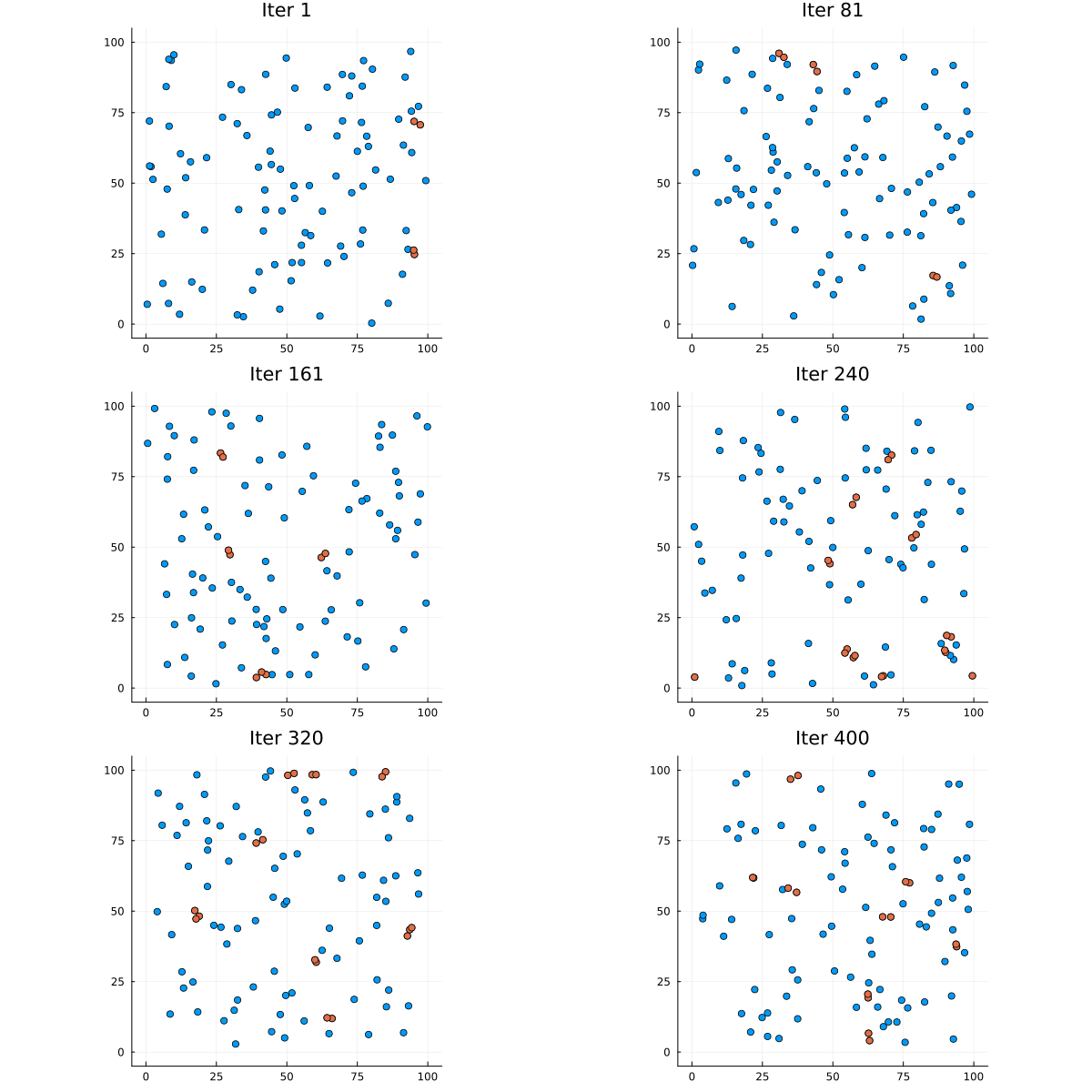
In this example, particles are moving with fixed velocity in a 2D space. The space is square but toroidal: that is to say that if a particle disappears off one edge it reappears on the opposite edge. The only behavioral complexity is that if two particles get too close to each other, their headings are reset at random.

Doing it in Julia

While the toroidal real space is built-in to NetLogo, it is easy to reproduce in other languages, by simply wrapping around coordinates with a modulo:

x = mod(x + delta_x, 100)
y = mod(y + delta_y, 100)

The particles can be considered objects, with x- and y-coordinates and a heading. This is also built-in to NetLogo but Julia has many options. I chose to represent them as mutable structs:

mutable struct Particle
    x
    y
    heading
end

Some utility functions:

• Get the NxN matrix of Euclidean distances between the N particles

function getdists(particlelist)
    nparticles = length(particlelist)
    dist = zeros(Float64, nparticles, nparticles)
    for i in 1:nparticles, j in i+1:nparticles
        dist[i,j] = dist[j,i] = sqrt((particlelist[i].x - particlelist[j].x)^2 + (particlelist[i].y - particlelist[j].y)^2)
    end
    return(dist)
end

• Identify all particles within a radius of a given particle

function ninradius(indiv, radius, particlelist, distances)
    neighbours = (1:length(particlelist))[distances[indiv,:] .< radius]
end

Initialisation: set the number of particles to 100, and create 100 of them, with random coordinates between 0 and 100, and a random heading. Speed is implicitly 1 unit per iteration.

nparticles = 100
particles = [Particle(rand()*100, rand()*100, rand()*2*pi) for i in 1:nparticles]

Julia’s animation framework

The main code body uses Julia’s convenient animation framework (part of the Plots.jl library), which allows the plot created in each pass through a loop to be combined into an animation object. The code body starts by (re-)calculating the inter-particle distances, and then for each particle, checks how many other particles are within 2 units. If there are any, that particle’s index is stored in clashlist, and its heading is changed at random.

Then each particle’s new location is calculated, from its present coordinates and newly re-calculated heading.

The final action of the loop is to create a plot: a scatterplot of the locations of all particles, overlaid by a scatter of those in the clashlist, so that we can see the impacts.

using Plots

anim = @animate for iter in 1:400
    dists = getdists(particles)
    # Update headings: change randomly if too close to another
    clashlist = []
    for i in 1:nparticles
        nlist = ninradius(i, 2, particles, dists);
        if length(nlist)>1
            particles[i].heading = rand()*2*pi
            push!(clashlist, i)
        end
    end

    # Update positions
    for i in 1:nparticles
        particles[i].x = mod(particles[i].x+cos(particles[i].heading), 100)
        particles[i].y = mod(particles[i].y+sin(particles[i].heading), 100)
    end

    scatter([particle.x for particle in particles],
            [particle.y for particle in particles], label=false, aspect_ratio = :equal, title="Iter $iter",
            xlims=(-5,105),ylims=(-5,105) )
    scatter!([particle.x for particle in particles[clashlist]],
             [particle.y for particle in particles[clashlist]], label=false)
end

gif(anim, fps=24, "particles.gif")

Conclusion

Compared with the Smaldino’s NetLogo code for the example (on GitHub), the Julia code is likely more demanding, but not longer or more verbose. NetLogo is designed for this specific class of task, whereas Julia is a general purpose language. However, with a knowledge of Julia it is quite easy to replicate this exercise, and we have immediate access to all the power of Julia in other areas (here the Plots library with its animation capacity is very helpful, but there are lots of other libraries which could support analysis of the data generated by the simulation).

In terms of code length, the NetLogo example file has over 500 lines, but less than 70 seem to be code written for this specific example. The Julia code has less than 55 lines. I’m not sure I have exactly replicated Smaldino’s example, but I think I have reproduced the main features.

NetLogo is a perfectly valid choice. Presenting an easier beginning allows students to concentrate on the simulation concepts more than the coding details. However, as long as I can depend on the incoming students having had some exposure to Julia (e.g., for data analysis), it is a more powerful option.

Postscript

Jonathan Carroll @jonocarroll@fostodon.org has written a tidier, more idiomatic version, at https://gist.github.com/jonocarroll/8180c068fa46fb3a3be4d7bbf0fd146f