The role of indelcost: OM, LCS and Hamming
How do you parameterise Optimal Matching analysis of lifecourse sequence data? A lot of ink has been spilt on how to build the substitution matrix, defining the differences between the states through which sequences move (the cost of substituting elements), but what about the role of indelcost, the cost of inserting or deleting elements? Here is a quick demonstration (using SADI, in Stata) that shows that below a certain threshold OM becomes LCS, the longest-common-subsequence distance measure, that above another threshold (less well-defined) it reverts to Hamming distance, and that in between there is a minimum meaningful indelcost. Let’s look at how this works (for equal-length sequences, since Hamming requires this; OM and LCS can also applied to sequences of unequal lengths).
The indel operation is what allows OM to detect similarity displaced in time, and the substitution operation to carry out comparison (displaced or otherwise). The Hamming distance does not use indels, and compares using substitution costs only, strictly without displacement. The LCS measure does not use substitution costs – elements are either the same or different – but does use insertions/deletions.
By inspecting the OM algorithm we can see that if the indelcost is less than half the maximum substitution cost, that maximum substitution will never be used, as an insert/delete pair will be cheaper (any substitution costing more than twice the indelcost will be ignored). Thus, if we respect the substitution matrix, the minimum indelcost is half the maximum substitution. This is a floor where OM has its greatest ability to recognise displaced similarity; higher values will make indels less likely, making displacement more costly.
In theory, LCS does not use substitution costs. But we can use OM code to estimate LCS, because if we set the indelcost to half the minimum substitution cost, the algorithm will in effect ignore the substitution operation. This gives us a second landmark on the indelcost terrain: less than half the minimum substitution cost gives LCS, between half the min and half the max, the substitution matrix is more or less truncated, at half the max we have the most displacing OM.
One more landmark, but one that depends on the actual data and not just the algorithm: if the indelcost is raised sufficiently, indels become so expensive that they do not occur, and OM reverts to the Hamming distance.
Let’s explore with a little code (see below for all code in one block):
First, set up: load the MVAD data, create a theoretically informed substitution matrix, mvdanes, and a “flat” one, flat, where all off-diagonal values are 1
use mvad
sort id

matrix mvdanes = (0,1,1,2,1,3 \ ///
                  1,0,1,2,1,3 \ ///
                  1,1,0,2,1,2 \ ///
                  2,2,2,0,1,1 \ ///
                  1,1,1,1,0,2 \ ///
                  3,3,2,1,2,0 )

sdmksubs, subsmat(flat) dtype(flat) nstates(6)
With the flat matrix, and an indelcost of 0.5, we use oma to generate the LCS distance. With the mvdanes matrix, and an effectively infinite indelcost (i.e., 999 is large enough in the context to guarantee indels are not used), we calculate the Hamming distance. While we’re at it, we also calculate the XTS distance (combinatorial duration-weighted subsequence count)1:
oma state1-state72, subsmat(flat)    pwd(lcs) length(72) indel(0.5)
oma state1-state72, subsmat(mvdanes) pwd(ham) length(72) indel(999)

cal2spell, state(state) spell(sp) length(len) nsp(nspells)
local spmax = r(maxspells)
combinadd sp1-len`spmax', pwsim(xts) nspells(nspells) nstates(6) rtype(d)
The business code comes next: for indelcost values between 0 and 4 we recalculate the OM distance (with the mvdanes matrix), and correlate the result with the three initial distances. We post the results to a postfile, which we can access afterwards:
postfile pf indel rho1 rho2 rho3 using omlcsham, every(1)

forvalues indeli = 0/100 {
    oma state1-state72, subsmat(mvdanes) pwd(oma) length(72) indel(`=`indeli'/25')
    corrsqm ham oma, nodiag
    local rho1 = r(rho)
    corrsqm lcs oma, nodiag
    local rho2 = r(rho)
    corrsqm xts oma, nodiag
    local rho3 = r(rho)
    post pf (`=`indeli'/25') (`rho1') (`rho2') (`rho3')
  }
}

postclose pf
Interpretation
Let’s graph the results:
use omlcsham, clear
label var rho1 "Hamming"
label var rho2 "LCS"
label var rho3 "XTS"
line rho* indel if indel<=4, xline(0.5 1.5) ///
title("OM's correlation with other measures, as indelcost varies") ///
note("MVAD data; subs-costs between 1 and 3")
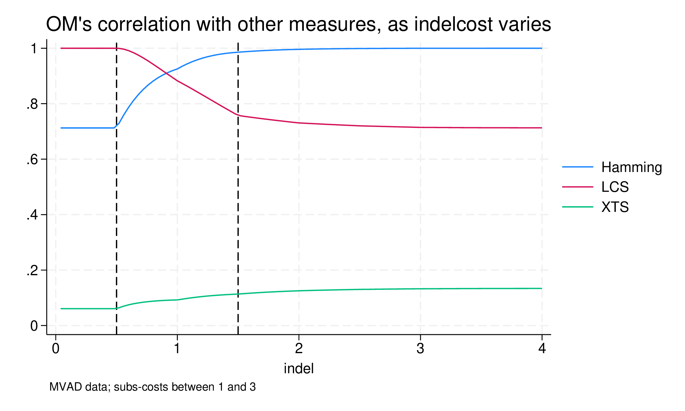
For the lowest values of indelcost, 0.0 to 0.5, the results are the same. The correlation between OM and LCS is 1.0, in other words, the results are identical, despite the different substitution matrices. This is to be expected, but it is nice to demonstrate that if the indelcost is less than or equal to the minimum substitution cost, substitutions are ignored. In this range the correlation with Hamming is 0.72.
In the range between 0.5 and 1.5 (half the min to half the max) everything changes. As indelcost rises, the effective substitution matrix changes from the flat matrix to the mvdanes one. Most change occurs in this range: above 1.5 things are not constant but vary much less. In this much we can see how LCS differs from OM and Hamming mostly because of the substitution operation, the recognition that some state pairs are more similar than others.
At 1.5, the correlation between OM and Hamming is already 0.985. That is, the difference in the estimated distance due to sensitivity to displaced similarity is really quite small. As is often the case, for many pairs of life-course sequences, displaced similarity does not matter, and for some it makes a very small difference. However, from a research point of view, where it does matter it is often very interesting: even with a correlation as high as this the clustering results will not be the same, and the interesting pairs of sequences will likely be clustered differently2
It is instructive to see how the OM/Hamming difference reacts as indelcost rises:
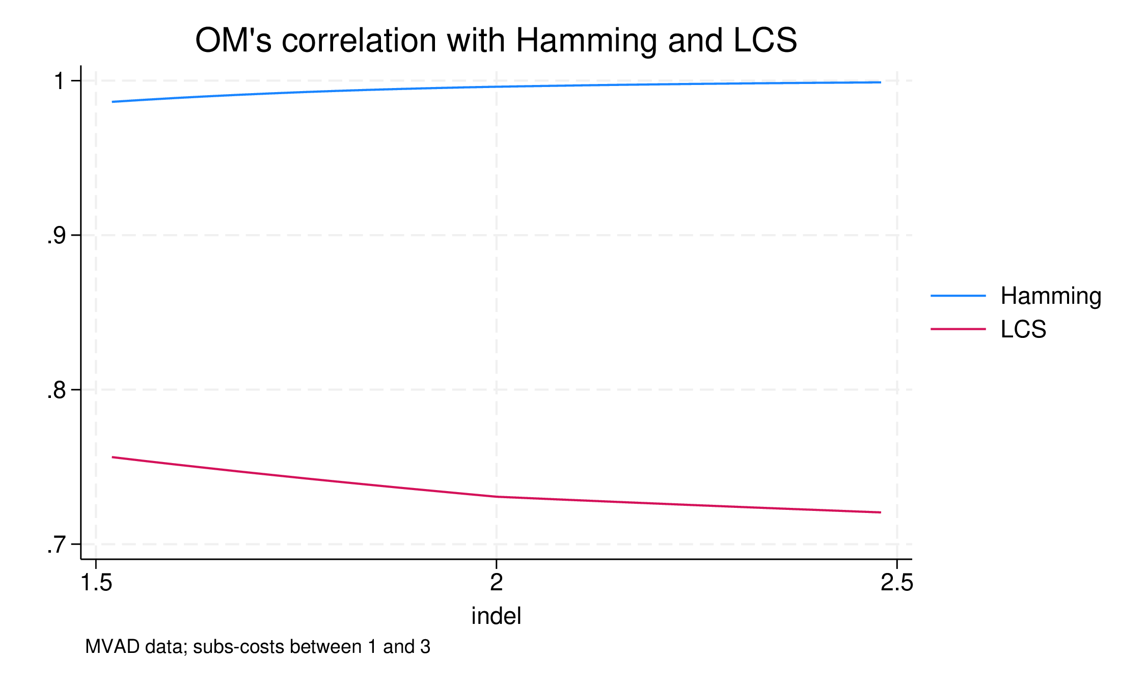
At 1.5, the correlation is 0.985, and it converges slowly on 1.0. In fact, with indelcost = 4.0, the correlation is 0.99998: almost there but there are still pairs where OM recognises displaced similarity, even at this high price.
Conclusion
OM, LCS and Hamming all belong to the same family of sequence analysis distance measures. As displacement becomes expensive, OM converges on Hamming. If we are to respect the substitution matrix, which matters for OM and Hamming, but not LCS, the minimum value of indelcost and the maximum freedom to recognise displaced similarity is half the maximum substitution cost. If we reduce indelcost below this, we begin to truncate the higher values of the substitution matrix, and OM converges on LCS. For indelcost less than or equal to half the minimum substitution cost, the substitution matrix is completly flattened and the OM distance is identical with LCS.
| Indelcost | Detection of similarity | Substitution costs |
|---|---|---|
| Very high | No displacement, OM converges on Hamming | Only substitution matters |
| Lower but >= half max subs-cost | OM recognises displaced similarity | Substitution matrix 100% respected |
| Half max subs-cost | OM maximally recognises displaced similarity | Substitution matrix 100% respected |
| Between half max and half min | Displaced similarity even more detected | Matrix truncated |
| <= half min subs-cost | Displaced exact matches detected | Matrix irrelevant |
Appendix
Code
use mvad
sort id

// Use the substitution matrix from the MVAD paper
matrix mvdanes = (0,1,1,2,1,3 \ ///
                  1,0,1,2,1,3 \ ///
                  1,1,0,2,1,2 \ ///
                  2,2,2,0,1,1 \ ///
                  1,1,1,1,0,2 \ ///
                  3,3,2,1,2,0 )

sdmksubs, subsmat(flat) dtype(flat) nstates(6)
// Get pairwise distance matrices for a range of different distance measures

oma state1-state72, subsmat(flat)    pwd(lcs) length(72) indel(0.5)
oma state1-state72, subsmat(mvdanes) pwd(ham) length(72) indel(999)

cal2spell, state(state) spell(sp) length(len) nsp(nspells)
local spmax = r(maxspells)
combinadd sp1-len`spmax', pwsim(xts) nspells(nspells) nstates(6) rtype(d)

postfile pf indel rho1 rho2 rho3 using omlcsham, every(1)

forvalues indeli = 0/100 {
    oma state1-state72, subsmat(mvdanes) pwd(oma) length(72) indel(`=`indeli'/25')
    corrsqm ham oma, nodiag
    local rho1 = r(rho)
    corrsqm lcs oma, nodiag
    local rho2 = r(rho)
    corrsqm xts oma, nodiag
    local rho3 = r(rho)
    post pf (`=`indeli'/25') (`rho1') (`rho2') (`rho3')
  }
}

postclose pf
Getting SADI
The calculations are done using SADI, my Stata package for sequence analysis. To install:
net from http://teaching.sociology.ul.ie/sadi
net install sadi, replace
net get sadi
The net get sadi command pulls the MVAD data (and other ancillary files) and saves it in the current folder as mvad.dta