Using Julia to plot OSM data

Posted on Oct 3, 2025

Plotting OSM data

There’s an awful lot of data on OpenStreetMap, and while the best place to look at it is on the map, it can also be downloaded and worked on offline. I wanted to do this with Julia, and actually made surprisingly quick progress.

How to

One way of accessing the data is via the good people at https://download.geofabrik.de/. They make OSM data available in ESRI shapefile format, inter alia. (You can also talk directly to the OSM databases, but that’s for another project.) I started by downloading the data for Ireland at https://download.geofabrik.de/europe/ireland-and-northern-ireland.html. The resulting archive contains sets of files relating to a number of themes (waterways, roads, buildings, natural features), but I extracted the roads one, specifially the files gis_osm_roads_free_1.shp and gis_osm_roads_free_1.dbf. These are respectively a shapefile (polygons) and a file of attributes for each feature, in a standard GIS format.

Julia can cope with this data via the Shapefile.jl library. Do import Pkg; Pkg.add("Shapefile") and you’re good to go (it pulls in the required GeoInterface library automatically, and what follows requires the Plots library). Activate it all as follows, and read in the data

using Shapefile, GeoInterface, Plots


table = Shapefile.Table("gis_osm_roads_free_1.shp")

class = table.fclass

Objects and functions

Everything ends up in the table object. The array table.geometry contains the traces for all the objects in the file, and table.fclass lists what each object is (here, the type of road or path, such as “motorway”, “trunk” or “cycleway”). Looking up table.fclass is slow, so it’s better to copy its contents to an array once, and use that.

Each element of table.geometry contains an array of latitude and longtitude pairs, extractable via GeoInterface.coordinates(), so we could plot one like this:

trace = GeoInterface.coordinates(table.geometry[1])[1]
lon = [x[1] for x in trace]
lat = [x[2] for x in trace]
plot(lon, lat)

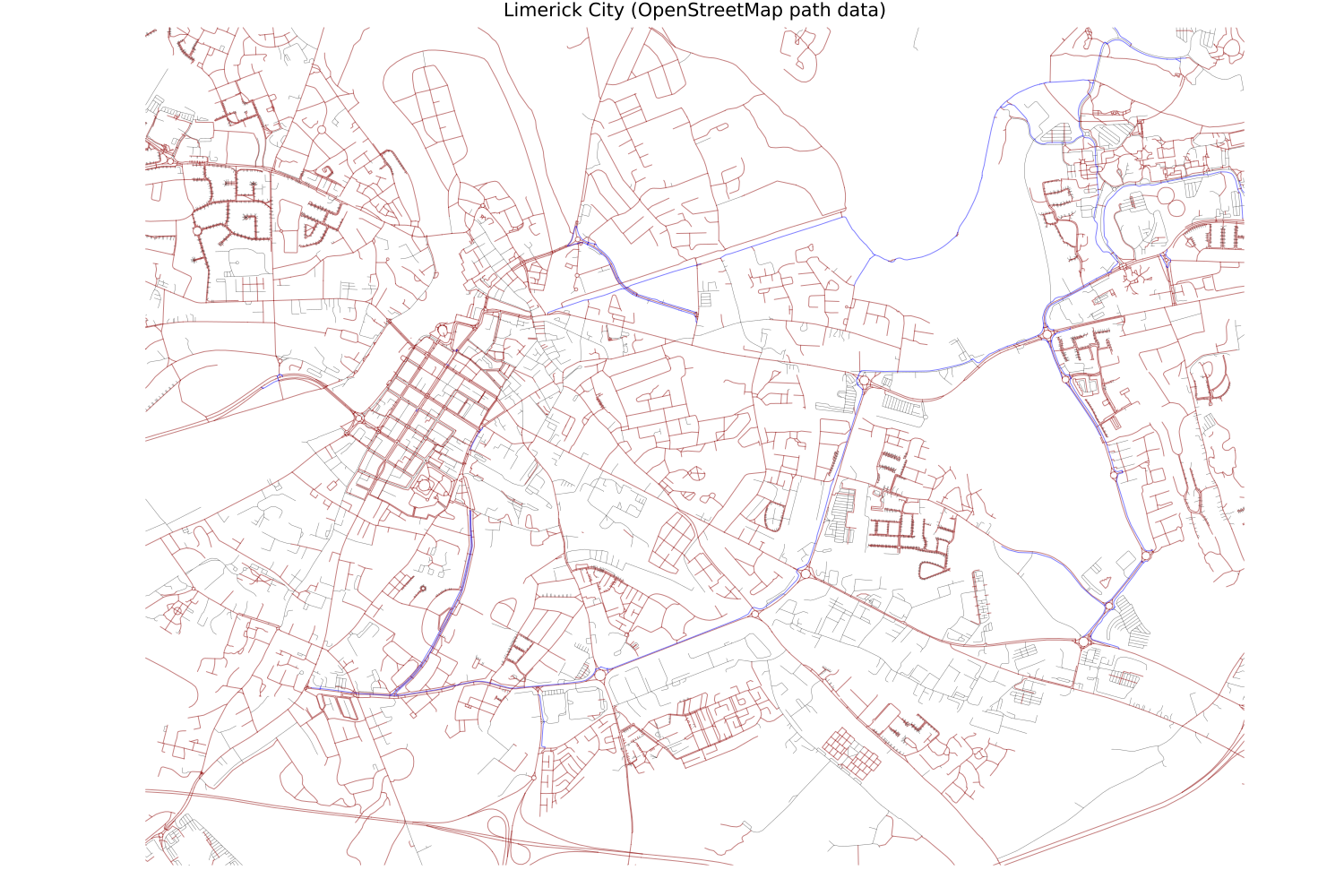
Plotting single paths is not interesting: there are 100s of 1000s of them. To many to plot, in fact, so we either need to select a rare type (e.g., motorways) and plot it for the whole island, or restrict ourselves to a fairly small bounding box (e.g., plot the paths for the city I live in, Limerick). If using a bounding box, we need to restrict ourselves to paths that have at least one point within it. This function does that (could be made more efficient for long paths, I’m sure):

function inbb(coords, minlat, maxlat, minlon, maxlon)
    # add test that BBs don't overlap, for speed?
    # if max(coord_lat)<minlat or min(coord_lat)>maxlat, or ditto for lon, skip loop.
    result = false
    for i in 1:size(coords)[1]
        if (minlon <= coords[i][1] <= maxlon) & (minlat <= coords[i][2] <= maxlat)
            result = true
            break
        end
    end
    return result
end

Another occasion for a function is the plotting code: if we’re going to plot multiple paths, we might as well tidy up the code. This function takes a path, its type (motorway, secondary, cycleway, etc.), the current plot identifier, and a bounding box. It then extracts the latitude and longitude arrays from the path, and adds them to the current plot (with different colour and linewidth according to path type). It only plots paths that enter within the bounding box (inbb()) and uses xlim and ylim in the plots to cut off paths as they exit the bounding box.

function plotpoly(element, fclass, p, minlat, maxlat, minlon, maxlon)
    trace = GeoInterface.coordinates(element)[1] # Is there always only one? In this data, yes.
    lon = [x[1] for x in trace]
    lat = [x[2] for x in trace]
    if inbb(trace, minlat, maxlat, minlon, maxlon)
        if (fclass == "service") | (fclass == "unclassified")
            plot!(p, lon, lat, color="black", alpha=0.5, label=false, linewidth=0.5, xlim=(minlon, maxlon), ylim=(minlat, maxlat))
        elseif fclass == "cycleway"
            plot!(p, lon, lat, color="blue", alpha=0.5, label=false, linewidth=1, xlim=(minlon, maxlon), ylim=(minlat, maxlat))
        else
            plot!(p, lon, lat, color="darkred", alpha=0.5, label=false, linewidth=1, xlim=(minlon, maxlon), ylim=(minlat, maxlat))
        end
    end
end

Main code

Then we come to the main code: first, create a new plot, p. Then iterate through all the table.geometry entries, applying plotpoly() to them. Finally, tidy up the plot: drop the axes and grid, and set the aspect ratio to approximately 1/cos(52°) to correct for that degrees of longitude represent much smaller distances than degrees of latitude, at this latitude.

p = plot(size=(1500,1000))

for i in 1:length(table.geometry)
    plotpoly(table.geometry[i], class[i], p, 52.64, 52.68, -8.65,-8.565) #50, 56, -11, -5.0)
end

plot!(p, aspect_ratio = 1.62, axis=false, grid=false, title="Limerick City (OpenStreetMap path data)")

Postscript

While the Shapefile.jl library is quite powerful (and general with respect to GIS), it is likely that it is more efficient to extract and plot OSM data with OSMMakie.jl.