Parameterising TWED
Time Warp Edit Distance (TWED) is a measure for comparing categorical time-series such as life-course sequences, that is designed to recognise similarity that may be displaced in time. It is similar to Optimal Matching distance in implementation, but can be thought of as locally compressing and stretching the time dimension, whereas OM deletes and inserts elements. TWED, OM and a range of other sequence comparison tools are implemented for Stata in my SADI package (see Appendix: code). How does TWED compare with other measures, and how does its parameterisation matter?
Lambda and nu
Like OM or the simpler Hamming distance, TWED uses a substitution-cost matrix to weight differences between states. Additionally, it has stiffness and gap parameters, nu and lambda, which control how likely the algorithm is to recognise similarity displaced in time. OM has an indelcost parameter (for the same purpose); Hamming has none, and can only recognise similarity that is not displaced in time.
This note reports a quick exercise to compare TWED and other distance measures, to understand the effect of the nu and lambda parameters. The measures used are
- OM with minimal indelcost (maximal ability to detect displaced similarity)
- Hamming distance (similarity at the same time only)
- Longest common subsequence length
- Elzinga’s duration-weighted count of common subsequence measures (spell-oriented)
Values of nu and lambda between 0.0 and 2.0 are considered. The sequences used are drawn from the example MVAD data set, distributed with SADI and TraMineR. For OM, Hamming and TWED, the following substitution matrix is used (based on the McVicar/Anyadike-Danes paper):
matrix mvdanes = (0,1,1,2,1,3 \ ///
                  1,0,1,2,1,3 \ ///
                  1,1,0,2,1,2 \ ///
                  2,2,2,0,1,1 \ ///
                  1,1,1,1,0,2 \ ///
                  3,3,2,1,2,0 )
For OM, the indelcost is set at 1.5, half the maximum substitution cost (values below this mean the higher values in the substitution cost matrix are not used; this value maximises the ability to detect similarity displaced in time). Hamming distance is estimated using OM with an indelcost of 999 (a value high enough that indels are not used). LCS is estimated with OM, using a “flat” substitution cost matrix (all off-diagonal values are constant) and an indelcost of half that constant. The XTS subsequence count distance is calculated with SADI’s combinadd command.
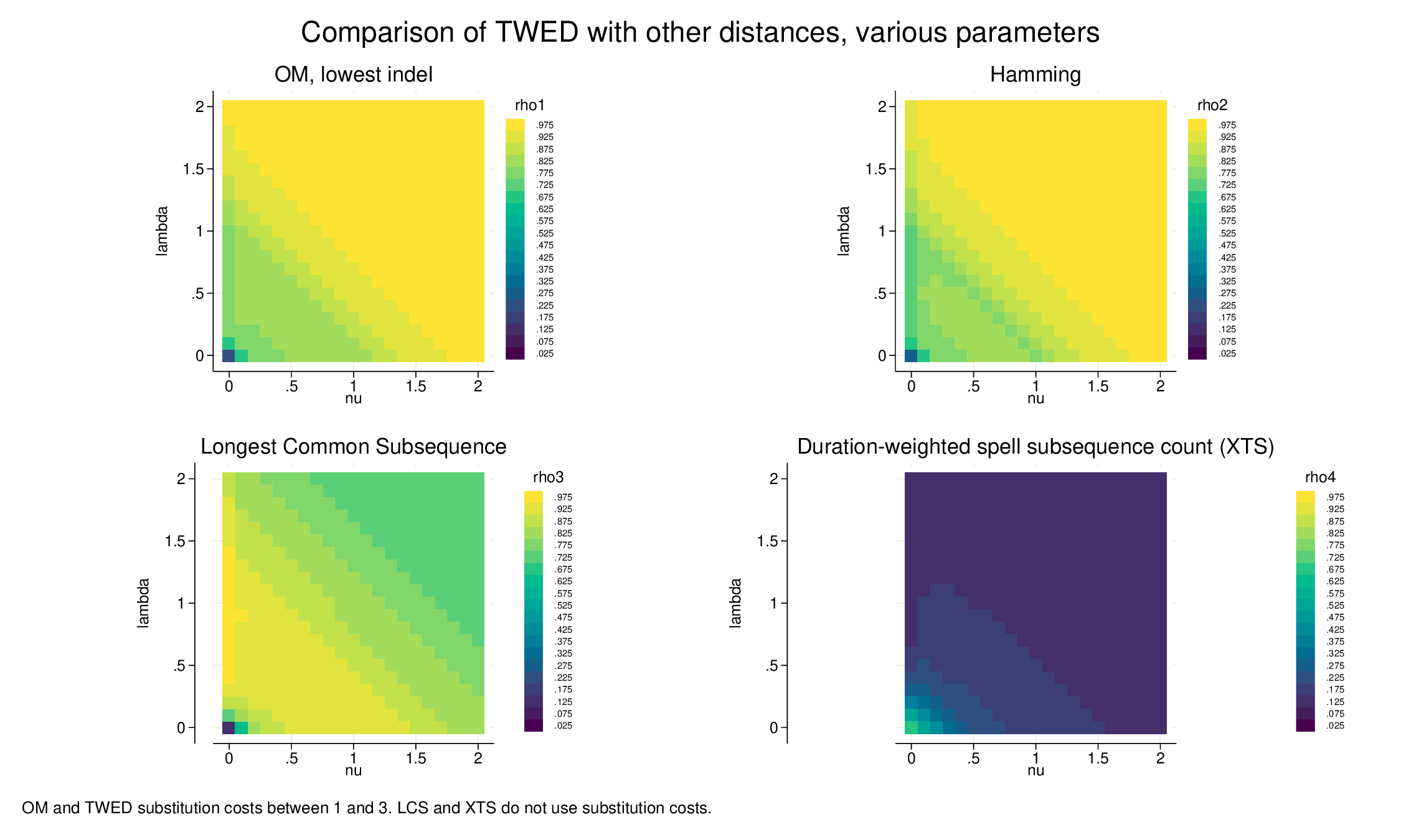
The measure considered is the correlation between the TWED distance and each of the reference distances. I use Ben Jann’s heatplot command to summarise the results:

OM and Hamming show very similar pictures (in fact, OM and Hamming are highly correlated, though where they differ is often informative). Effectively, TWED with high values of nu and lambda (in particular, high values of their sum, of nu+lambda) yields very similar distances. At lower values of nu+lambda, the correlation is moderate, and at very low values it drops precipitately. There are slight differences between OM and Hamming but overall the similarity is remarkable.
LCS, the Longest Common Subsequence measure, has some similarity, notably the very low correlation at the minimum nu+lambda values. However, it has distinctly higher correlations at moderate values of nu+lambda, and correlations drop off modestly as nu and lambda increase towards the max.
XTS (which as a distance measure has a radically different logic) has almost no correlation with TWED, except at the very lowest values of nu+lambda.
Interpretation
At high values of nu+lambda, TWED distances are very similar to OM and Hamming using the same substitution costs. As the parameter values drop, TWED is picking up a different sort of similarity. In fact, at lower values of nu+lambda (about 0.5 to 1.5), TWED is more similar to LCS, despite LCS not using a substitution matrix1. Interestingly, for the lowest values of nu+lambda, TWED is similar only to XTS (if only moderately so). In summary, as far as this exercise goes (and results can be expected not to be identical with different data), TWED is reflecting the substitution cost structure at higher values of the parameters, at lower values is doing something similar to LCS, and at the lowest values is similar to the duration-weighted spell-focused XTS measure.
nu+lambda
The nu and lambda parameters are usually described as controlling stiffness and gap penalties, but in the main the patterns respond to their sum, and not to each parameter differently (i.e., the heatmaps display diagonal patterns). The systematic exception to this pattern is at nu=0, where the effect of lambda differs in all four panels.
Appendix: code
Getting SADI
The calculations are done using SADI, my Stata package for sequence analysis. To install:
net from http://teaching.sociology.ul.ie/sadi
net install sadi, replace
net get sadi
The net get sadi command pulls the MVAD data (and other ancillary files) and saves it in the current folder as mvad.dta
Create the data
use mvad
sort id

// Use the substitution matrix from the MVAD paper
matrix mvdanes = (0,1,1,2,1,3 \ ///
                  1,0,1,2,1,3 \ ///
                  1,1,0,2,1,2 \ ///
                  2,2,2,0,1,1 \ ///
                  1,1,1,1,0,2 \ ///
                  3,3,2,1,2,0 )

// "Flat" substitution matrix
sdmksubs, subsmat(flat) dtype(flat) nstates(6)

// Get pairwise distance matrices for a range of different distance measures
oma state1-state72, subsmat(mvdanes) pwd(omd15) length(72) indel(1.5)
oma state1-state72, subsmat(flat)    pwd(lcs)   length(72) indel(0.5)
oma state1-state72, subsmat(mvdanes) pwd(ham)   length(72) indel(999)

// Setup for Elzinga's combinatorial XTS measure
cal2spell, state(state) spell(sp) length(len) nsp(nspells)
local spmax = r(maxspells)
combinadd sp1-len`spmax', pwsim(xts) nspells(nspells) nstates(6) rtype(d)

postfile pf lambda nu rho1 rho2 rho3 rho4 using twedsim2, every(1)

forvalues lambdai = 0/20 {
  forvalues nuj = 0/20 {
    twed state1-state72, subsmat(mvdanes) pwd(twd_`lambdai'_`nuj') length(72) ///
      lambda(`=`lambdai'/10') nu(`=`nuj'/10')
    corrsqm omd15 twd_`lambdai'_`nuj', nodiag
    local rho1 = r(rho)
    corrsqm ham  twd_`lambdai'_`nuj', nodiag
    local rho2 = r(rho)
    corrsqm lcs   twd_`lambdai'_`nuj', nodiag
    local rho3 = r(rho)
    corrsqm xts twd_`lambdai'_`nuj', nodiag
    local rho4 = r(rho)
    post pf (`=`lambdai'/10') (`=`nuj'/10') (`rho1') (`rho2') (`rho3') (`rho4')
  }
}

postclose pf
Draw the graph
use twedsim2
heatplot rho1 lambda nu, aspect(1) discrete(0.1) name(gr1, replace) title("OM, lowest indel") cuts(0(0.05)1.0)
heatplot rho2 lambda nu, aspect(1) discrete(0.1) name(gr2, replace) title("Hamming") cuts(0(0.05)1.0)
heatplot rho3 lambda nu, aspect(1) discrete(0.1) name(gr3, replace) title("Longest Common Subsequence") cuts(0(0.05)1.0)
heatplot rho4 lambda nu, aspect(1) discrete(0.1) name(gr4, replace) ///
  title("Duration-weighted spell subsequence count (XTS)") cuts(0(0.05)1.0)
graph combine gr1 gr2 gr3 gr4, scale(0.7) title("Comparison of TWED with other distances, various parameters") ///
  note("OM and TWED substitution costs between 1 and 3. LCS and XTS do not use substitution costs.")
A second data set
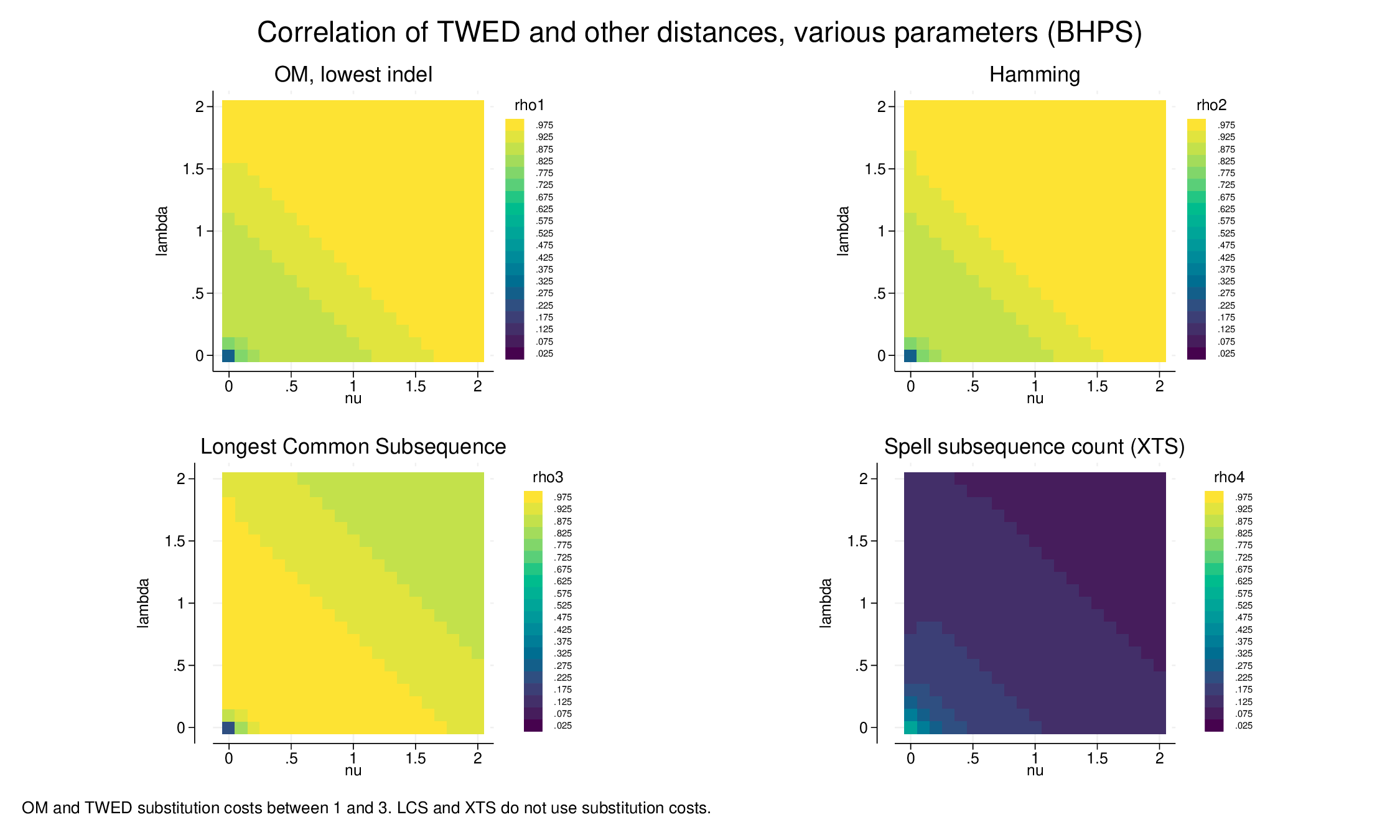
For comparison, doing a similar exercise on mothers’ labour market histories (BHPS data) yields consistent results. There there are four states, full-time work, part-time, unemployed, non-employed, and a linear substitution matrix. The correlations with OM, Hamming and LCS may be a little higher, but the effects of the parameterisation is similar.

References
- The original description of SADI is in the Stata Journal (2017): https://journals.sagepub.com/doi/pdf/10.1177/1536867X1701700302
- TWED and other measures are compared and discussed in a book chapter (2014): https://link.springer.com/chapter/10.1007/978-3-319-04969-4_5 (paywalled) or https://www.ul.ie/media/31080/download?inline (earlier version)
-
In practice, LCS can be estimated in SADI by using OM, with an indelcost less than or equal to half the lowest substitution cost. With this setting, indel operations are always favoured to substitutions ↩︎