No, your variable doesn't need to be normally distributed

“I need to test my variables for normality”

I keep encountering students (mostly with former exposure to business or psych stats) who insist on testing their variables for normality as a sine qua non prior to conducting analysis. While it’s clearly a good idea to have a sense of how your variables are distributed, normality is (a) not a general requirement and (b) rarely the case (if your tests tell you the variable is normal, it’s most likely because your N is too small).

What is important is using a model that suits the data (and the question) and complying with the requirements of that model. For models that are based on OLS (i.e., linear regression, and ANOVA) the assumption is that the residuals are approximately normally distributed (and in practice, unimodal symmetric is good enough). If your Y-variable is discrete, or might have a non-linear (e.g., multiplicative) relationship with the X-variables, use something other than OLS.

The other place normality comes into play is in sampling distributions. Standard statistical inference starts with the Central Limit Theorem which states that for any sufficiently large samle, the sampling distribution of a sample statistic will be approximately normal. Two things to note: (a) the sampling distribution of a statistic is a very different thing to the empirical distribution of a variable, and (b) we’re already aware of the need for “sufficiently large” samples (and have specific small-sample backups for particular cases, such as the t, binomial and chi-sq distributions).

But seeing this behaviour again recently set me thinking. Exactly how much does normality matter? Do simple analyses like the humble t-test behave better with normally distributed data? The Central Limit Theorem suggests that this should not be the case with big samples, but does performance decay differently as sample size declines?

To test this, I created a small simulation in Stata: it creates data where the null hypothesis is true, i.e., groups A and B are drawn from the same (specifiable) distribution, and then runs a t-test on the A-B difference. We do this repeatedly, and count how often the confidence interval around the estimate contains the true value. If approximately 2.5% of cases fall below the 95% interval and 2.5% above, performance is good; otherwise it is problematic.

Results

The following distributions are used:

• normal
• uniform (platykurtic)
• logistic (fatter tails, leptokurtic)
• log-normal (right skewed)
• Bernoulli (two equally likely values)

The code is below, and you can use it with any distribution supported by Stata.

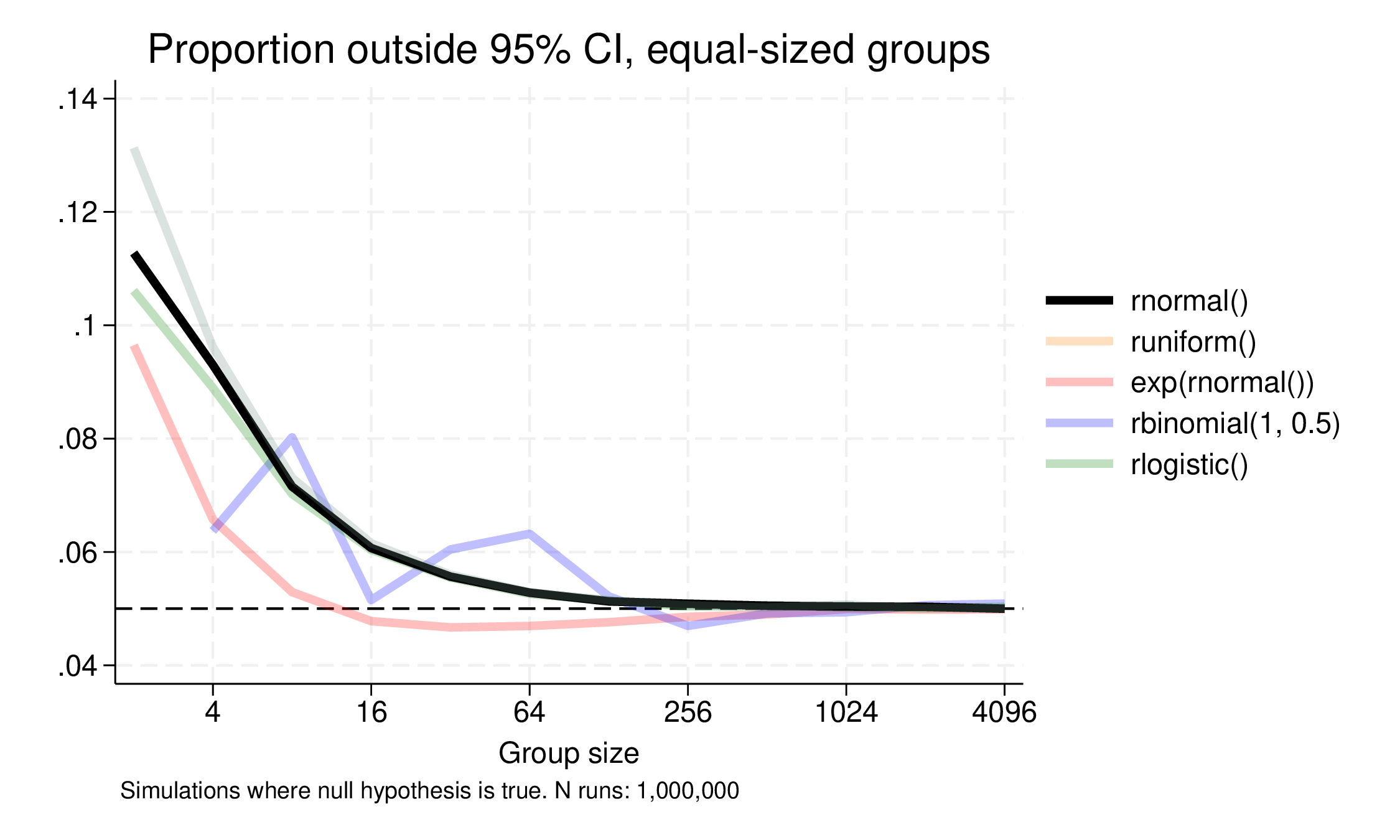
We try with equal group sizes, from 2 to 4096, and the results are here:

Normal, uniform and logistic distribution results are pretty similar, with the Bernoulli looking a bit erratic at lower Ns, but perhaps surprisingly the skewed log-normal distribution does best, staying close to the 95% coverage down to two groups of 8. In fact, what is possibly surprising is how poorly even normally distributed variables do at even moderately small sample sizes (and the non-normally symmetric distributions also). At two groups of 16, coverage is down to 94%, 93% at two groups of 8. (The Bernoulli or binomially distributed case is weird because the sampling distribution is discrete and this matters a lot at small sample sizes.)

The takeaway is that normality doesn’t really help much:

• performance is poor at small sample sizes
• little or no better than other symmetric distributions
• in fact poorer than the right skewed distribution.

Focus on the logic of your model, not the normality of your Y-variable.

Code

program funccov, rclass
syntax, FUN(string) [NTreat(integer 100) NControl(integer 100) NSamp(integer 1000) CLEAR]
if "`clear'" != "" {
  clear
}

local N =`ntreat'+`ncontrol'
local tcrit = invt(`N'-2, 0.975)

qui {
  set obs `=`N'*`nsamp''
  gen group = 1 + int((_n-1)/`N')
  bysort group: gen treat = _n <= int(`ntreat')
  gen x = `fun'
  collapse (mean) xm = x (sd) xsd=x, by(group treat)
  reshape wide xm xsd, i(group) j(treat)
  gen d = xm0 - xm1
  gen sdc = sqrt((xsd0^2*(`ntreat'-1) + xsd1^2*(`ncontrol'-1))/(`ntreat'+`ncontrol'+1))
  gen se = sqrt(sdc^2/`=`ntreat'' + sdc^2/`=`ncontrol'')
  gen tstat = d/se
  count if (tstat > `tcrit') & (tstat!=.)
  local hi = r(N)
  count if (tstat < -`tcrit') & (tstat!=.)
  local lo = r(N)
  count if tstat!=.
  local nvalid = r(N)
}

di "Threshold: " `tcrit'
di "Sample size: " `N' ", group 1: " `ntreat' ", group 2: " `ncontrol'
di "Number of runs: " `nvalid'
di %20s "`fun'" %8.5f `=`lo'/`nvalid'' %8.5f `=`hi'/`nvalid''
return scalar lo = `lo'/`nvalid'
return scalar hi = `hi'/`nvalid'
end


postfile pf lo hi nt nc ns str32 func using runsimeq, every(5) replace

local ns 10000
forvalues iter = 1/100 {
  forvalues nt = 1/12 {
    local ng = 2^`nt'
    foreach f in "rnormal()" "runiform()" "exp(rnormal())" "rbinomial(1, 0.5)" "rlogistic()" {
      funccov, nt(`ng') nc(`ng') nsamp(`ns') fun(`f') clear
      post pf (r(lo)) (r(hi)) (`ng') (`ng') (`ns') ("`f'")
    }
  }
}

postclose pf